Denoising
Contents
Show code cell content
# My tools: sets the path and adds some math macros for LaTeX equations
# Needs internet access to install.
try:
    import mmf_setup
    mmf_setup.nbinit()
except ImportError:
    import sys
    !{sys.executable} -m pip install --user --upgrade mmf-setup
    print("Restart your kernel and try again")
This cell adds /home/docs/checkouts/readthedocs.org/user_builds/iscimath-583-learning-from-signals/checkouts/latest/src to your path, and contains some definitions for equations and some CSS for styling the notebook. If things look a bit strange, please try the following:
- Choose "Trust Notebook" from the "File" menu.
- Re-execute this cell.
- Reload the notebook.
Show code cell content
# Initialize plotting:
%matplotlib inline
# Import numpy and matplotlib.  These aliases are quite standard
import numpy as np, matplotlib.pyplot as plt
import scipy.stats
sp = scipy
# Suppress some logging messages in Pillow (Python Imaging Library)
import logging; logging.getLogger('PIL').setLevel(logging.ERROR)  # Suppress PIL messages
/home/docs/checkouts/readthedocs.org/user_builds/iscimath-583-learning-from-signals/conda/latest/lib/python3.9/site-packages/scipy/__init__.py:146: UserWarning: A NumPy version >=1.16.5 and <1.23.0 is required for this version of SciPy (detected version 1.23.5
  warnings.warn(f"A NumPy version >={np_minversion} and <{np_maxversion}"
Denoising#
The Problem#
Given some data \(d\) obtained by adding noise to an original image \(u_0\), how can we best approximate \(u\)? In this assignment, we will explore approximations \(u_\lambda\) obtained from the minimization problem
where \(\eta\) is (approximately) gaussian noise with standard deviation \(\eta\).
We call \(E[u]\) the “energy”, and in the following, normalize it by \(E[d]\) so that the noisy image has energy \(E[d]=1\).
import denoise

sigma = 0.4
lam = 0.1
im = denoise.Image()
d = denoise.Denoise(image=im, sigma=sigma, lam=lam)
u_exact = im.get_data(sigma=0)
u_noise = im.get_data(sigma=sigma)
u = d.minimize(callback=None)
E_u = d.get_energy(u)
E_noise = d.get_energy(u_noise)
E_exact = d.get_energy(u_exact)
fig, axs = denoise.subplots(3)
for _u, title, ax in [(u_exact, rf"Original: $\sigma=0$, $E={E_exact:.2g}$", axs[0]),
                     (u_noise, rf"Data: $\sigma={sigma}$, $E={E_noise:.2g}$", axs[1]),
                     (u, rf"$u_{{{lam}}}$: $\lambda={lam}$, $E={E_u:.2g}$", axs[2])]:
    im.show(_u, ax=ax)
    ax.set(title=title);
# Try to find an approximation u from u_noise
Walkthrough#
Loading Images#
# See what images are available

!ls images/
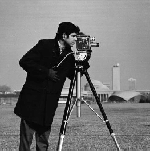
The-original-cameraman-image.png
Use the Python Imaging Library (PIL) to load images:
# Use the PIL to load the image
from PIL import Image

im = Image.open("images/The-original-cameraman-image.png")
im  # or display(im), but this happens by default for the last line
Adding Noise#
# First, see what the data looks like as an array.
# IMPORTANT: Convert to "L", "RGB" etc. or things get wierd:-)
# We also normalize pixel values in [0, 1)
u = u_exact = np.asarray(im.convert("L")) / 256
display(u)
display((u.shape, u.max(), u.min()))
print(f"{u.shape=}, {u.max()=}, {u.min()=}")  # Nicer python f-string
array([[0.97265625, 0.98046875, 0.98046875, ..., 0.98828125, 0.98046875,
        0.98828125],
       [0.62109375, 0.62109375, 0.62890625, ..., 0.59765625, 0.60546875,
        0.60546875],
       [0.61328125, 0.61328125, 0.61328125, ..., 0.59765625, 0.59765625,
        0.57421875],
       ...,
       [0.4765625 , 0.4921875 , 0.50390625, ..., 0.51171875, 0.51171875,
        0.4296875 ],
       [0.50390625, 0.50390625, 0.4921875 , ..., 0.51171875, 0.50390625,
        0.4140625 ],
       [0.95703125, 0.98046875, 0.98828125, ..., 0.97265625, 0.99609375,
        0.95703125]])
((490, 487), 0.99609375, 0.0)
u.shape=(490, 487), u.max()=0.99609375, u.min()=0.0
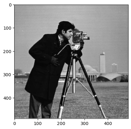
We see that the image is 490×487 in shape, and has unsigned integers ranging from 0 to 255.
# We can also display the array
plt.imshow(u, vmin=0, vmax=1, cmap="gray", interpolation=None)
<matplotlib.image.AxesImage at 0x7f1e5c4e25b0>
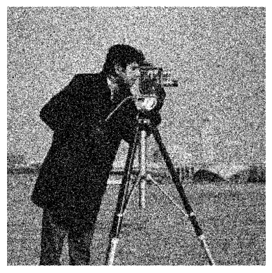
# Use random numbers to add noise.  Here we get a random number generator (rng)
# and use a fixed seed so we can reproduce our results
rng = np.random.default_rng(seed=2)
sigma = 0.3
u_noise = u + sigma * rng.normal(size=u.shape)
plt.imshow(u_noise, vmin=0, vmax=1, cmap="gray")

# Turn off the axes
ax = plt.gca()
ax.axis("off");
Removing Noise#
def imshow(u):
    fig, ax = plt.subplots()
    im = ax.imshow(u, vmin=0, vmax=1, cmap='gray')
    return im
def laplacian(u):
    """Return the laplacian of the image usings unit spacing."""
    return sum(
        np.gradient(
            np.gradient(u, axis=_a, edge_order=2), axis=_a, edge_order=2)
        for _a in [0, 1])
    return (np.gradient(np.gradient(u, axis=0), axis=0) +
            np.gradient(np.gradient(u, axis=1), axis=1))

# This already exists, with better boundary condistion, in scipy:
import scipy.ndimage
import scipy as sp

def laplacian(u):
    return sp.ndimage.laplace(u)
from ipywidgets import interact

d2u = laplacian(u_exact)

#@interact(p=(0, 50, 1))
def go(p=10):
    "Explore percentile thresholding of laplacian"
    fig, axs = plt.subplots(1, 2)
    for ax, u in zip(axs, [u_exact, u_noise]):
        d2u = laplacian(u)
        vmin, vmax = np.percentile(d2u, [p, 100-p])
        ax.imshow(d2u, vmin=vmin, vmax=vmax, cmap='gray')
        ax.axis("off")
We will minimize
where \(d\equiv\)u_noise is the data, or the noisy image. We can do this with a
direct gradient descent:
from scipy.integrate import solve_ivp

beta = 1.0
lam = 1.0  # Lam

def compute_E(u, lam=lam):
    """Return the energy."""
    E_regularization = (-u * laplacian(u)).sum()
    E_data_fidelity = (np.abs(u-u_noise)**2).sum()
    print(f"{E_regularization=}, {E_data_fidelity=}")
    return E_regularization + lam * E_data_fidelity

def compute_dy_dt(t, y, beta=beta, lam=lam):
    """Return dy_dt."""
    # solve_ivp expects y to be 1D, so we need to reshape
    u = y.reshape(u_noise.shape)
    du = 2*(-laplacian(u) + lam * (u - u_noise))
    dy = np.ravel(- beta * du)
    return dy


# Make initial guess 1D.  We start with the noise.
y0 = np.ravel(u_noise)
dT = 10
res = solve_ivp(compute_dy_dt, y0=y0, t_span=(0, dT))
u1 = res.y[:, -1].reshape(u_noise.shape)
plt.imshow(u1, vmin=0, vmax=1, cmap='gray')
<matplotlib.image.AxesImage at 0x7f1e5bf2f7c0>

from functools import partial
from IPython.display import clear_output
import tqdm

dT = 1
lam = 0.001  # Lam
lam = 1/2.2  # Lam
steps = 10

err0 = (np.abs(u_noise - u_exact)**2).mean()
E0 = compute_E(u_noise, lam=lam)

errs = []
Es = []
ts = []
y = y0
t = 0
fig, ax = plt.subplots()
for step in tqdm.tqdm(range(steps)):
    res = solve_ivp(partial(compute_dy_dt, beta=beta, lam=lam), y0=y, t_span=(t, t+dT))
    y = res.y[:, -1]
    u = y.reshape(u_noise.shape)
    errs.append((np.abs(u - u_exact)**2).mean()/err0)
    Es.append(compute_E(u, lam=lam)/E0)
    t = res.t[-1]
    ts.append(t)
    ax.cla()
    ax.imshow(u, vmin=0, vmax=1, cmap='gray')
    clear_output(wait=True)
    display(fig)
plt.close('all')
100%|██████████| 10/10 [00:04<00:00, 2.50it/s]
100%|██████████| 10/10 [00:04<00:00, 2.50it/s]
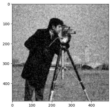
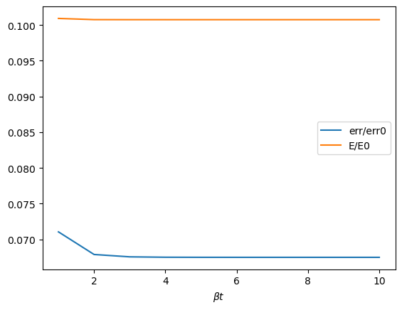
fig, ax = plt.subplots()
ax.plot(ts, errs, label='err/err0')
ax.plot(ts, Es, label='E/E0')
ax.legend()
ax.set(xlabel=r"$\beta t$");  # Python r-string
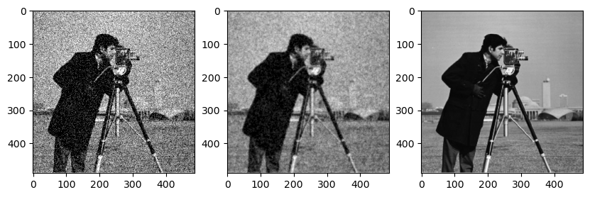
fig, axs = plt.subplots(1, 3, figsize=(10, 5))
ax = axs[0]
ax.imshow(u_noise, vmin=0, vmax=1, cmap="gray")
ax = axs[1]
ax.imshow(u, vmin=0, vmax=1, cmap="gray")
ax = axs[2]
ax.imshow(u_exact, vmin=0, vmax=1, cmap="gray")
<matplotlib.image.AxesImage at 0x7f1e5bbe02e0>
Exploration#
Here we explore some properties of denoising using the tools in denoise.py, which
packages code similar to that use above into classes and functions for easy reuse,
testing, and exploration.
We start with an image and various levels of noise. Here we normalize the images to have values between \(0\) (black) and \(1\) (white). The noise is normally distribute \(\eta \sim \mathcal{N(0, \sigma)}\) with standard deviation \(\sigma\) with values truncated so that the pixel values remain between \(0\) and \(1\), so the resulting noise is not exactly gaussian, but is truncated in a way that depends on the value of the pixels in the image.
%matplotlib inline
import numpy as np, matplotlib.pyplot as plt
import scipy.stats
sp = scipy
import PIL
from importlib import reload
import denoise;reload(denoise)

im = denoise.Image()
sigmas = np.linspace(0, 1, 6)
fig, axs = plt.subplots(1, len(sigmas), figsize=(len(sigmas)*2, 2))
for sigma, ax in zip(sigmas, axs):
    plt.sca(ax)
    im.imshow(im.get_data(sigma=sigma))
    ax.set(title=f"{sigma=:.2g}")
If we did not truncate the pixel values to remain in \([0, 1]\), then the following image of the noise term would be completely random. The truncation leaves an imprint of the image for large values of \(\sigma\):
sigma = 0.4
fig, axs = denoise.subplots(2, height=5)
im = denoise.Image()
u_exact = im.get_data(sigma=0)
u_noise = im.get_data(sigma=sigma)
du = u_noise - u_exact
im.show(du, ax=axs[1])
ax = axs[0]
ax.hist(du.ravel(), bins=100, density=True);
x = np.linspace(-1, 1, 500)
ax.plot(x, sp.stats.norm(scale=sigma).pdf(x))
[<matplotlib.lines.Line2D at 0x7f1e5bcd4250>]
Now we try denoising \(\sigma=0.4\) with various values of \(\lambda\):
import denoise;reload(denoise)
from IPython.display import clear_output, display
sigma = 0.4
lams = [0.01, 0.1, 1, 10]
im = denoise.Image()
d = denoise.Denoise(image=im)

fig, axs = denoise.subplots(2+len(lams), height=3)

for label, u, ax in [("Original", d.u_exact, axs[0]),
                     ("Noise", d.u_noise, axs[-1])]:
    im.show(u, ax=ax)
    ax.set(title=f"{label}: E={d.get_energy(u):.2g}")

display(fig)
for lam, ax in zip(lams, axs[1:-1]):
    d = denoise.Denoise(image=im, sigma=sigma, lam=lam, mode="wrap")
    u = d.solve()
    im.show(u, ax=ax)
    ax.set(title=f"{lam=:.2g}, E={d.get_energy(u):.2g}")
    clear_output(wait=True)
    display(fig)
plt.close('all')
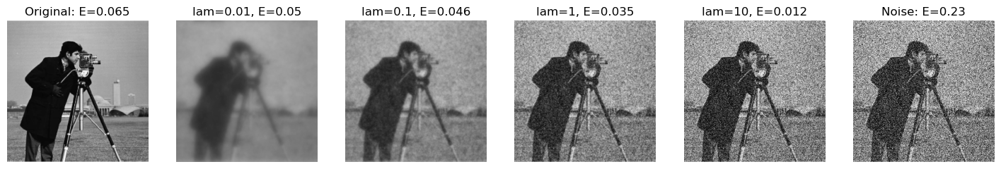
Ideas to Explore#
From the previous figure, it is clear that the parameter \(\lambda\) somehow controls the “energy”. Can you make this dependence explicit (using properties of both \(u_0=\)
u_exactand \(d=\)u_noise).Express the minimization problem in terms of a Bayesian problem. How does the truncation of the errors alter this analysis?
Fourier Techniques#
Here we try to directly implement the Fourier inversion technique discussed in class.
%matplotlib inline
from IPython.display import clear_output
import numpy as np, matplotlib.pyplot as plt
import denoise

sigma = 0.4
lam = 0.1

im = denoise.Image()
d = denoise.Denoise(image=im, sigma=sigma, lam=lam)

Nx, Ny = im.shape
dx = dy = 1.0
x = (np.arange(Nx) * dx)[:, None]
y = (np.arange(Ny) * dy)[None, :]
kx = 2 * np.pi * np.fft.fftfreq(Nx, dx)[:, None]
ky = 2 * np.pi * np.fft.fftfreq(Ny, dy)[None, :]

fft, ifft = np.fft.fftn, np.fft.ifftn

u = ifft(lam * fft(d.u_noise) / (lam + (kx**2 + ky**2)))
assert np.allclose(u.imag, 0)
u_fft = u.real
u_solve = d.minimize(d.u_noise)

clear_output()
data = [
    ("Original", d.u_exact),
    ("Noise", d.u_noise),
    ("FFT", u_fft),
    ("Minimize", u_solve),
]
fig, axs = denoise.subplots(len(data))
for ax, (title, u) in zip(axs, data):
    im.show(u, ax=ax)
    ax.set(title=title)
# Here is an interactive version

from ipywidgets import interact

#@interact(sigma=(0.0, 2.0), log_lam=(-10.0, 1.0))
def go(sigma=0.4, log_lam=-1):
    lam = 10**(log_lam)
    im = denoise.Image()
    d = denoise.Denoise(image=im, sigma=sigma, lam=lam, mode="wrap")

    Nx, Ny = im.shape
    dx = dy = 1.0
    x = (np.arange(Nx) * dx)[:, None]
    y = (np.arange(Ny) * dy)[None, :]
    kx = 2 * np.pi * np.fft.fftfreq(Nx, dx)[:, None]
    ky = 2 * np.pi * np.fft.fftfreq(Ny, dy)[None, :]

    fft, ifft = np.fft.fftn, np.fft.ifftn

    u = ifft(lam * fft(d.u_noise) / (lam + (kx**2 + ky**2)))
    assert np.allclose(u.imag, 0)
    u_fft = u.real

    data = [("Original", d.u_exact), ("Noise", d.u_noise), ("FFT", u_fft)]
    fig, axs = denoise.subplots(len(data), height=4)
    for ax, (title, u) in zip(axs, data):
        im.show(u, ax=ax)
        ax.set(title=title)
Source Code#
The following cells contain the source code for modules used in this document. They
need to be executed once to generate the source files, but afterwards can just be
imported. They use the %%writefile magic which writes the contents to file. We
will usually distribute this with the handout.
#%%writefile denoise.py
"""Module with tools for exploring image denoising.
"""
from functools import partial
import logging
import os.path
from pathlib import Path

import numpy as np
import matplotlib.pyplot as plt
import scipy.ndimage
import scipy.optimize

import PIL

logging.getLogger("PIL").setLevel(logging.ERROR)  # Suppress PIL messages

sp = scipy

plt.rcParams["image.cmap"] = "gray"  # Use greyscale as a default.


def subplots(cols=1, rows=1, height=3, **kw):
    """More convenient subplots that also sets the figsize."""
    args = dict(figsize=(cols * height, rows * height))
    args.update(kw)
    return plt.subplots(rows, cols, **args)


class Base:
    """Base class for setting attributes."""

    def __init__(self, **kw):
        for key in kw:
            if not hasattr(self, key):
                raise ValueError(f"Unknown {key=}")
            setattr(self, key, kw[key])
        self.init()

    def init(self):
        return


class Image(Base):
    """Class to load and process images."""

    if os.path.exists("images"):
        # Use a local directory if it exists.  Does not need mmf_setup
        dir = Path("images")
    else:
        # Otherwise (i.e. for documentation) go relative to ROOT
        import mmf_setup

        mmf_setup.set_path()
        dir = Path(mmf_setup.ROOT) / ".." / "_data" / "images"

    filename = "The-original-cameraman-image.png"
    seed = 2

    def init(self):
        self.rng = np.random.default_rng(seed=self.seed)
        self._filename = Path(self.dir) / self.filename
        self.image = PIL.Image.open(self._filename)
        self.shape = self.image.size[::-1]

    @property
    def rgb(self):
        """Return the RGB form of the image."""
        return np.asarray(self.image.convert("RGB"))

    def get_data(self, normalize=True, sigma=0, rng=None):
        """Return greyscale image.

        Arguments
        ---------
        normalize : bool
            If `True`, then normalize the data so it is between 0 and 1.
        sigma : float
            Standard deviation (as a fraction) of gaussian noise to add to the image.
            The result will be clipped so it does not exceed (0, 255) or (0, 1) if
            `normalize==True`.
        """
        data = np.asarray(self.image.convert("L"))
        vmin, vmax = 0, 255
        if normalize:
            data = data / vmax
            vmax = 1.0

        if sigma:
            if rng is None:
                rng = self.rng
            eta = sigma * rng.normal(size=data.shape)
            if normalize:
                data += eta
            else:
                data = vmax * eta + data
            data = np.minimum(np.maximum(data, vmin), vmax)
            if not normalize:
                data = data.round(0).astype("uint8")
        return data

    @property
    def data(self):
        """Return a greyscale image with data between 0 and 255."""
        return np.asarray(self.image.convert("L"))

    def __repr__(self):
        return self.image.__repr__()

    def _repr_pretty_(self, *v, **kw):
        return self.image._repr_pretty_(*v, **kw)

    def _repr_png_(self):
        """Use the image as the representation for IPython display purposes."""
        return self.image._repr_png_()

    def show(self, u, vmin=None, vmax=None, ax=None, **kw):
        if vmax is None:
            if u.dtype == np.dtype("uint8"):
                vmax = max(255, u.max())
            else:
                vmax = max(1.0, u.max())
        if vmin is None:
            vmin = min(0, u.min())

        if ax is None:
            ax = plt.gca()

        ax.imshow(u, vmin=vmin, vmax=vmax, **kw)
        ax.axis("off")

    imshow = show


class Denoise(Base):
    lam = 1.0
    mode = "reflect"
    image = None
    sigma = 0.5
    seed = 2

    def init(self):
        self.rng = np.random.default_rng(seed=self.seed)
        self.u_exact = self.image.get_data(sigma=0, normalize=True)
        self.u_noise = self.image.get_data(sigma=self.sigma,
                                           normalize=True,
                                           rng=self.rng)
        self._E_noise = self.get_energy(self.u_noise,
                                        parts=True,
                                        normalize=False)
        self._E_exact = self.get_energy(self.u_exact, parts=True)

    def laplacian(self, u):
        """Return the laplacian of u."""
        return sp.ndimage.laplace(u, mode=self.mode)

    def get_energy(self, u, parts=False, normalize=True):
        """Return the energy.

        Arguments
        ---------
        parts : bool
            If True, return (E, E_regularization, E_data_fidelity)
        normalize : bool
            If True, normalize by the starting values for u_noise.
        """
        u_noise = self.u_noise
        E_regularization = (-u * self.laplacian(u)).sum()
        E_data_fidelity = (abs(u - u_noise)**2).sum()
        E = E_regularization + self.lam * E_data_fidelity
        E0 = 1
        if normalize:
            E0 = self._E_noise[0]

        if parts:
            return (E / E0, E_regularization / E0, E_data_fidelity / E0)
        else:
            return E / E0

    def pack(self, u):
        """Return y, the 1d real representation of u for solving."""
        return np.ravel(u)

    def unpack(self, y):
        """Return `u` from the 1d real representation y."""
        return np.reshape(y, self.u_noise.shape)

    def compute_dy_dt(self, t, y):
        """Return dy_dt for the solver."""
        return -self.beta * self._df(y=y)

    def _f(self, y):
        """Return the energy"""
        return self.get_energy(self.unpack(y))

    def _df(self, y, u_noise=None):
        """Return the gradient of f(y)."""
        E0 = self._E_noise[0]
        u = self.unpack(y)
        return self.pack(2 * (-self.laplacian(u) + self.lam *
                              (u - self.u_noise))) / E0

    def callback(self, y, plot=False):
        u = self.unpack(y)
        E, E_r, E_f = self.get_energy(u, parts=True)

        msg = f"E={E:.2g}, E_r={E_r:.2g}, E_f={E_f:.2g}"
        if plot:
            import IPython.display

            fig = plt.gcf()
            ax = plt.gca()
            ax.cla()
            IPython.display.clear_output(wait=True)
            self.image.show(u, ax=ax)
            ax.set(title=msg)
            IPython.display.display(fig)
        else:
            print(msg)

    def minimize(self,
                 u0=None,
                 method="L-BFGS-B",
                 callback=True,
                 tol=1e-8,
                 plot=False,
                 **kw):
        if u0 is None:
            u0 = self.u_noise
        y0 = self.pack(u0)
        if callback:
            callback = partial(self.callback, plot=plot)
        res = sp.optimize.minimize(
            self._f,
            x0=y0,
            jac=self._df,
            method=method,
            callback=callback,
            tol=tol,
            **kw,
        )
        if not res.success:
            raise Exception(res.message)

        if plot:
            plt.close("all")
        u = self.unpack(res.x)
        return u